Introduction to QGIS:
QGIS, also known as Quantum GIS, is a user-friendly and feature-rich GIS software that enables users to create, edit, visualize, and analyse spatial data with ease. Developed by a global community of GIS enthusiasts and professionals, QGIS offers a robust set of tools and functionalities to support a wide range of GIS tasks, from simple mapping to complex spatial analysis.
QGIS, also known as Quantum GIS, is a user-friendly and feature-rich GIS software that enables users to create, edit, visualize, and analyse spatial data with ease. Developed by a global community of GIS enthusiasts and professionals, QGIS offers a robust set of tools and functionalities to support a wide range of GIS tasks, from simple mapping to complex spatial analysis.
User Interface and Navigation:
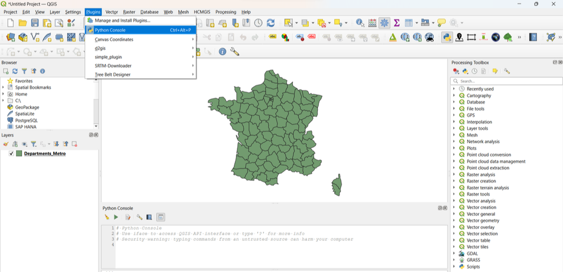
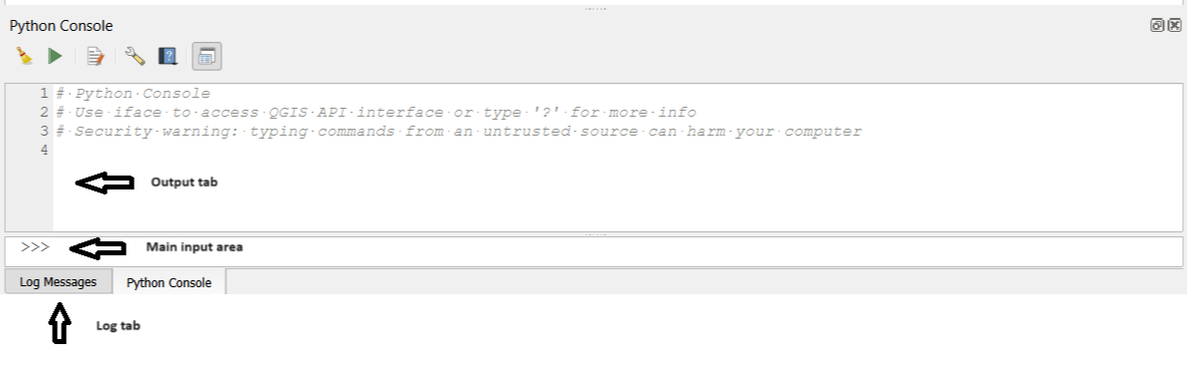
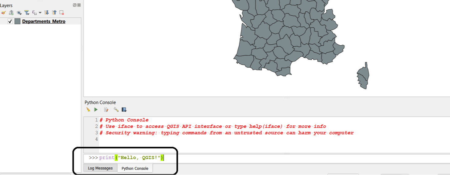
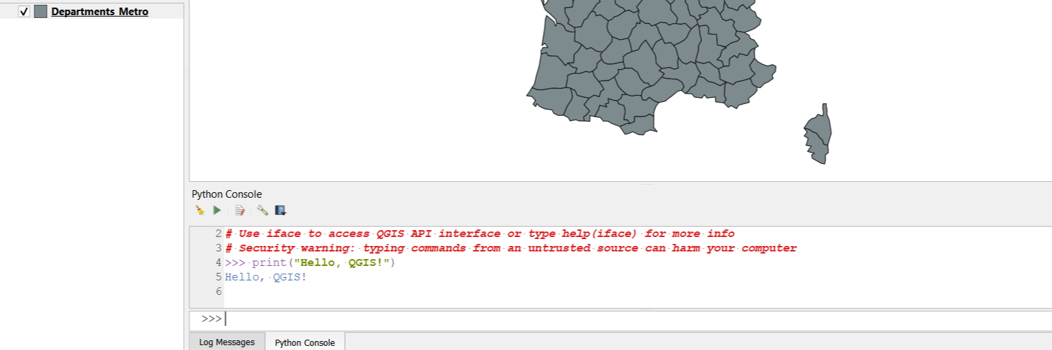
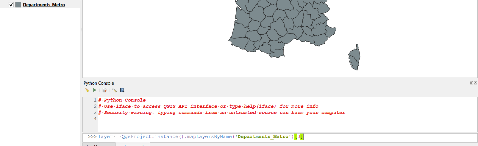
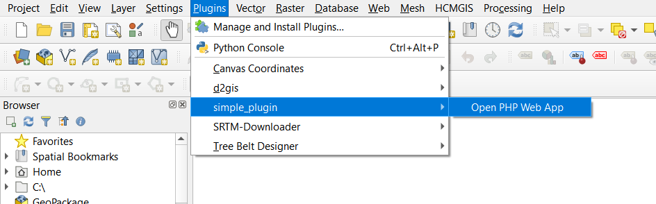
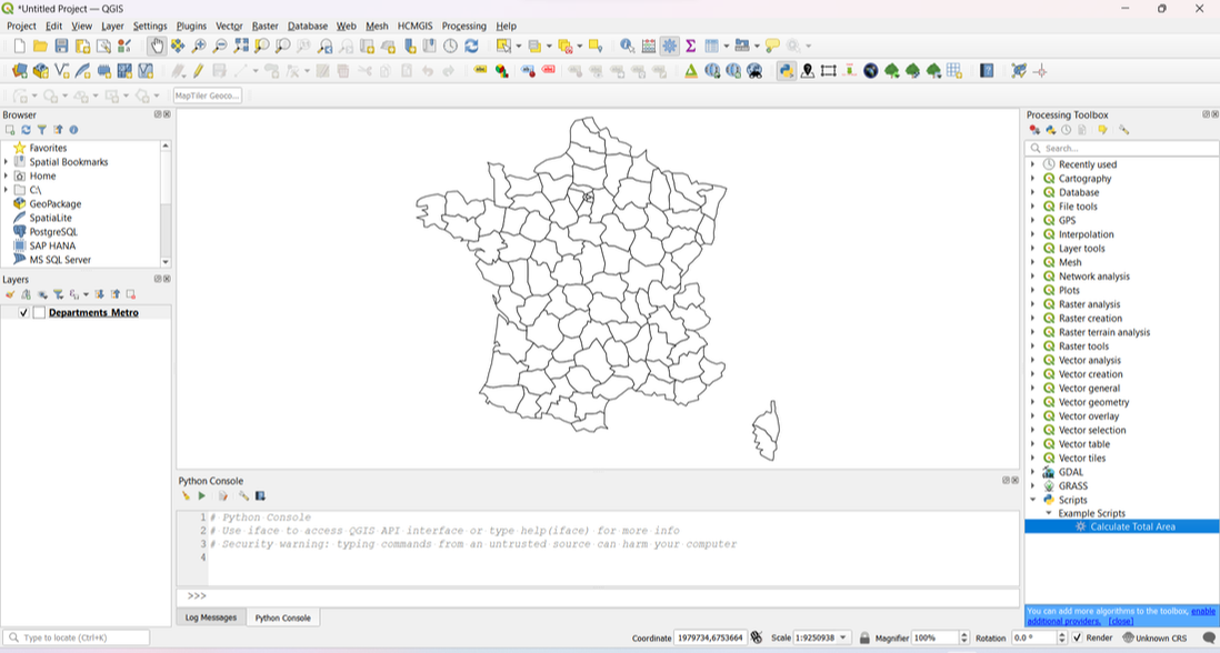
Upon launching QGIS, you'll be greeted with an intuitive user interface designed to facilitate seamless navigation and access to essential tools. The interface consists of various panels, including the Layers panel for managing spatial data layers, the Browser panel for browsing files and databases, and the Map Canvas for viewing and interacting with your maps. Familiarizing yourself with these components will help you navigate QGIS efficiently and make the most of its features.
Upon launching QGIS, you'll be greeted with an intuitive user interface designed to facilitate seamless navigation and access to essential tools. The interface consists of various panels, including the Layers panel for managing spatial data layers, the Browser panel for browsing files and databases, and the Map Canvas for viewing and interacting with your maps. Familiarizing yourself with these components will help you navigate QGIS efficiently and make the most of its features.
Importing and Managing Spatial Data:
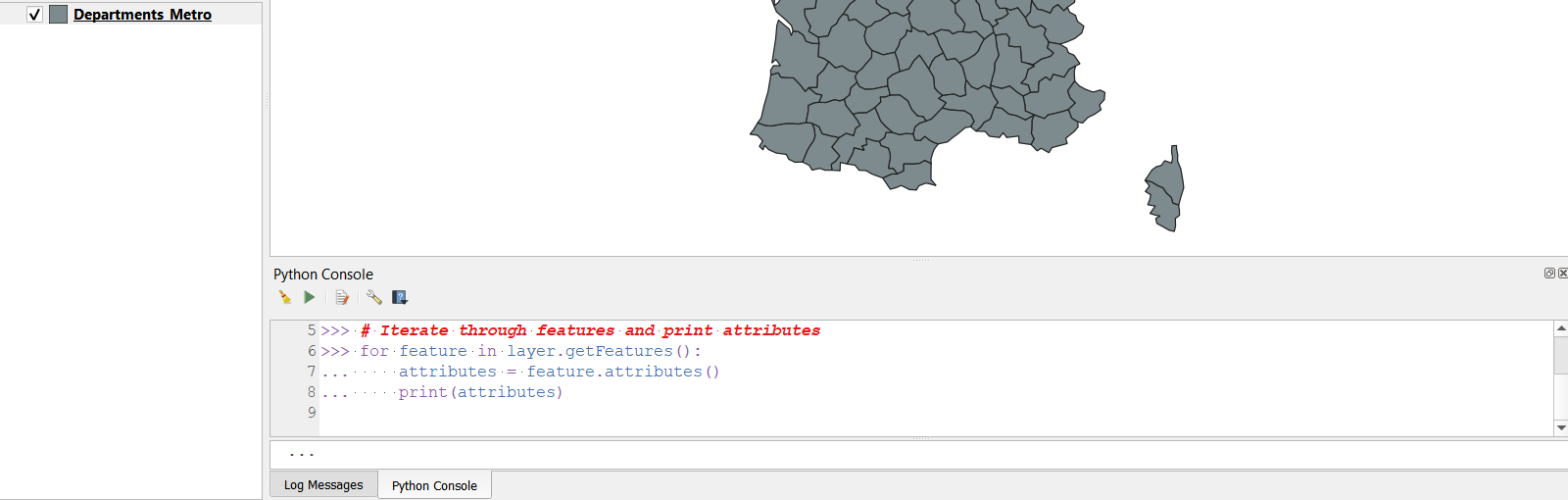
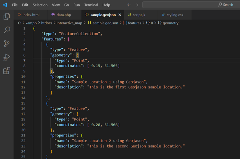
QGIS supports a multitude of spatial data formats, including shapefiles, GeoTIFFs, GPS data, and more, making it easy to import and manage your spatial data within the software. Whether you're working with data from a local file or connecting to a remote database, QGIS provides straightforward methods for importing, organizing, and editing your spatial datasets. Understanding how to effectively manage spatial data is essential for conducting meaningful analysis and creating informative maps.
QGIS supports a multitude of spatial data formats, including shapefiles, GeoTIFFs, GPS data, and more, making it easy to import and manage your spatial data within the software. Whether you're working with data from a local file or connecting to a remote database, QGIS provides straightforward methods for importing, organizing, and editing your spatial datasets. Understanding how to effectively manage spatial data is essential for conducting meaningful analysis and creating informative maps.
Mapping Tools and Cartographic Design:
One of the highlights of QGIS is its powerful mapping tools, which allow users to create visually compelling maps tailored to their specific needs. From basic symbology and labelling options to advanced cartographic features like scale-dependent rendering and map composer, QGIS provides the flexibility to design maps that effectively communicate spatial data insights. Learning how to leverage these mapping tools will enable you to create professional-quality maps that convey information accurately and effectively.
One of the highlights of QGIS is its powerful mapping tools, which allow users to create visually compelling maps tailored to their specific needs. From basic symbology and labelling options to advanced cartographic features like scale-dependent rendering and map composer, QGIS provides the flexibility to design maps that effectively communicate spatial data insights. Learning how to leverage these mapping tools will enable you to create professional-quality maps that convey information accurately and effectively.
Spatial Analysis Techniques:
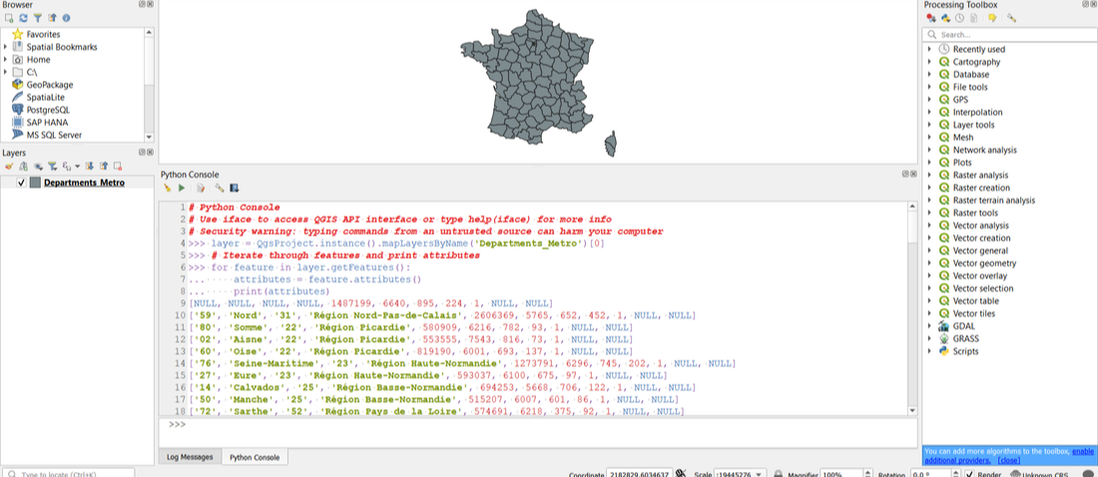
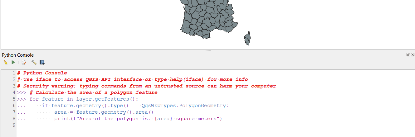
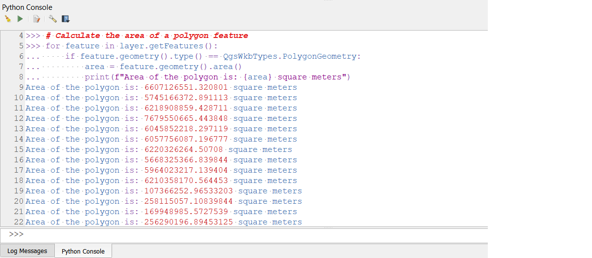
In addition to its mapping capabilities, QGIS offers a wide range of spatial analysis tools and functionalities to support data-driven decision-making. Whether you're conducting proximity analysis, spatial interpolation, or complex geoprocessing tasks, QGIS provides the tools and resources you need to perform meaningful spatial analysis. Mastering these spatial analysis techniques will empower you to extract valuable insights from your spatial data and address real-world challenges more effectively.
In addition to its mapping capabilities, QGIS offers a wide range of spatial analysis tools and functionalities to support data-driven decision-making. Whether you're conducting proximity analysis, spatial interpolation, or complex geoprocessing tasks, QGIS provides the tools and resources you need to perform meaningful spatial analysis. Mastering these spatial analysis techniques will empower you to extract valuable insights from your spatial data and address real-world challenges more effectively.
In conclusion, QGIS is a versatile and powerful GIS software that offers a wealth of features and capabilities for spatial data analysis and visualization. By familiarizing yourself with its user interface, mastering its mapping tools, and exploring its spatial analysis techniques, you can unlock the full potential of QGIS and embark on a rewarding journey of GIS exploration and discovery. Remember, learning GIS is a gradual process that requires patience, practice, and perseverance. So don't hesitate to dive in, experiment with different features, and seek guidance from experienced GIS professionals.


 RSS Feed