Geographic Information Systems (GIS) have become an integral part of modern-day decision-making processes, aiding in understanding, analysing, and presenting spatial data. One of the powerful tools in the GIS realm is QGIS Server, which allows you to serve maps and spatial data over the web. If you're new to the subject of communicating with QGIS Server using PHP, fear not, as this blog will provide you with a beginner-friendly introduction.

Understanding QGIS Server:
QGIS Server is an open-source software that enables you to publish your QGIS projects as web services. This means you can create interactive maps and provide access to your spatial data through web applications. It is built on top of the QGIS desktop application, allowing you to utilize your existing QGIS projects and share them online.

Why Use PHP with QGIS Server:
PHP (Hypertext Preprocessor) is a widely-used scripting language that's especially suited for web development. When combined with QGIS Server, PHP can be used to create dynamic web applications that interact with and display maps and spatial data. It acts as a bridge between the user interface and the QGIS Server backend.

Setting Up the Environment:
Before you start communicating with QGIS Server using PHP, you need to ensure you have the right environment set up. This involves having QGIS Server installed on a server along with PHP support. You can choose to install these components separately or use a pre-packaged solution like OSGeo4W, which bundles both QGIS Server and PHP.

Making Your First PHP and QGIS Server Interaction:
Let's take a simple example of how you can use PHP to communicate with QGIS Server and display a basic map on a web page.

Step 1: Connecting to QGIS Server:
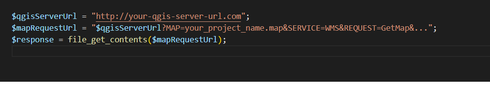
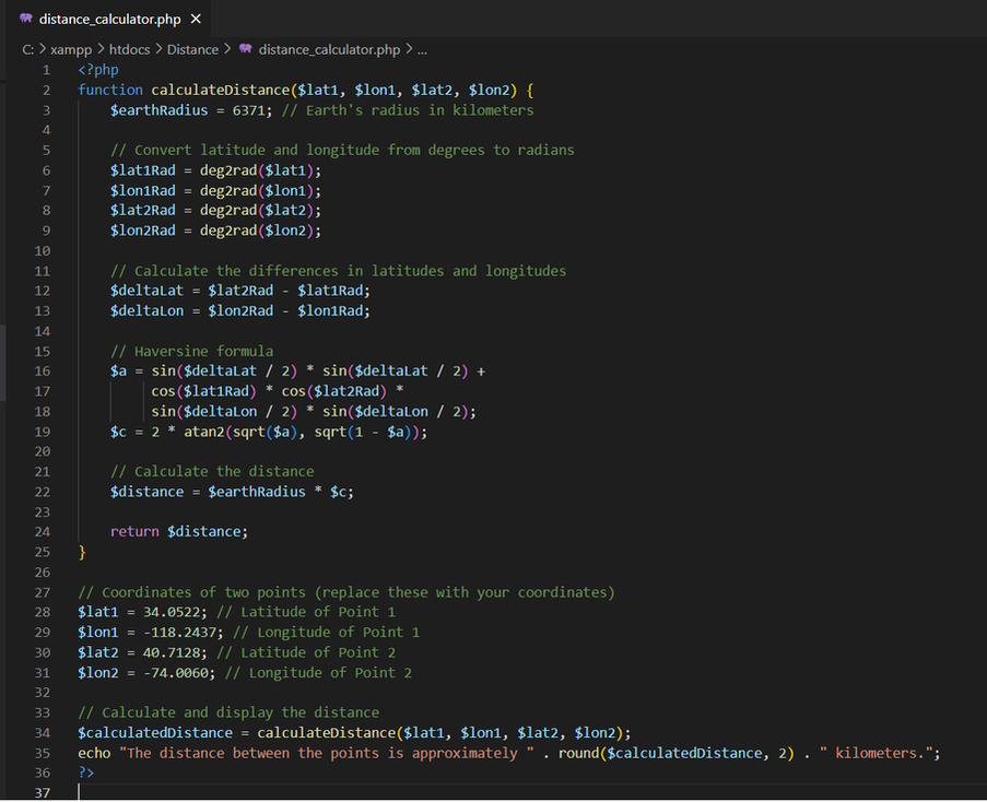
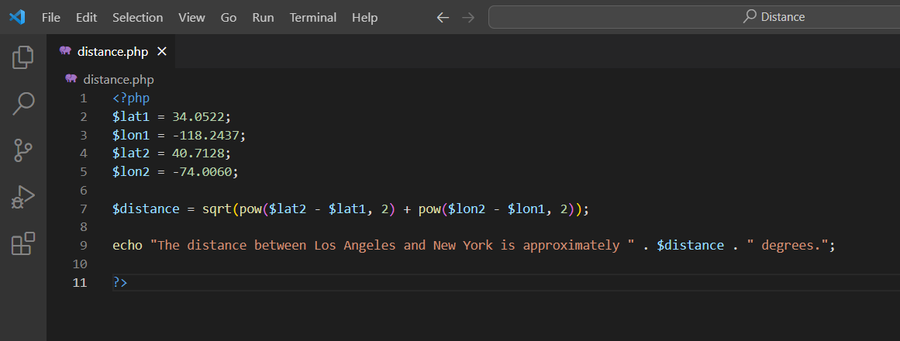
In your PHP file, you need to establish a connection to your QGIS Server using its REST API. This API allows you to request map images and other information. Use the `file_get_contents` function to make a request to the appropriate QGIS Server endpoint, like this:

Step 2: Displaying the Map:

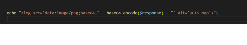
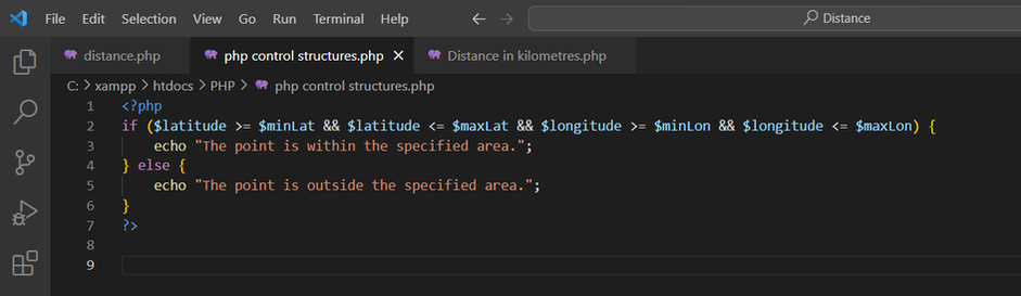
After getting the response from QGIS Server, you can display the map image on your web page. You can use the `<img>` HTML tag and set the `src` attribute to the data you received from QGIS Server:

Step 3: Enhancing Interaction:
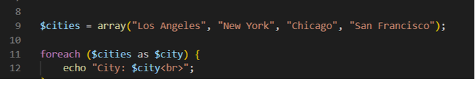
To create a more interactive experience, you can add parameters to your QGIS Server requests. For example, you can change the extent of the map, add layers, or change the output format.

Conclusion:
Communicating with QGIS Server using PHP opens up a world of possibilities for sharing and interacting with spatial data over the web. Whether you're creating simple map displays or building complex web GIS applications, understanding the basics of PHP-QGIS Server communication is a valuable skill. With this introductory knowledge, you're now equipped to explore more advanced features and create meaningful web-based GIS solutions.

In the realm of Geographic Information Systems (GIS), the fusion of spatial data and web technologies has given rise to dynamic geospatial web mapping. At the forefront of this revolution is the QGIS Server—an open-source solution that empowers GIS professionals and enthusiasts to share, publish, and interact with geospatial data through web applications. This blog serves as an introduction to the QGIS Server, shedding light on its capabilities and the endless possibilities it offers for geospatial data dissemination.

What is the QGIS Server?
The QGIS Server is a robust component of the QGIS suite—an open-source desktop GIS software. Unlike the QGIS desktop application, which focuses on creating, editing, and analysing geographic data, the QGIS Server specializes in serving this data to web clients. It allows users to access maps, perform spatial queries, and visualize data using a web browser interface.

Key Capabilities of the QGIS Server:
1. Web Map Publishing: The QGIS Server enables you to publish your QGIS projects as web maps that users can access remotely. This means you can share your geospatial insights with a global audience through a simple web interface.

2. Spatial Data Dissemination: The server offers a streamlined way to disseminate your spatial data to a broader audience. Whether you're presenting environmental data, city planning maps, or resource distribution, the QGIS Server simplifies access.

3. Customizable Web Maps: QGIS Server facilitates the creation of interactive and customizable web maps. You can enable users to toggle layers, zoom in on specific areas, and perform spatial analyses—all within the browser.

4. Geoprocessing Services: Beyond data visualization, the QGIS Server supports geoprocessing capabilities. Users can execute spatial analyses like buffering, clipping, and distance calculations directly through the web interface.

5. Open Standards: The server adheres to open web standards like OGC (Open Geospatial Consortium) protocols. This means compatibility with a wide range of web mapping clients and applications.

Getting Started with QGIS Server:
1. Install and Configure: Begin by setting up the QGIS Server on your chosen server environment. Configuration involves defining project paths, map layers, and access settings.

2. Publish Projects: Using QGIS Desktop, create your map projects with layers, styling, and symbology. Once prepared, you can publish these projects to the QGIS Server.

3. Access Web Maps: Users can access the published maps via a web browser. They can interact with the maps, query data, and explore geographic features.

QGIS Server: A Gateway to Geospatial Web Mapping:
In a world driven by data accessibility and visualization, the QGIS Server serves as a gateway to bring your geospatial insights to life. Whether you're an environmental scientist sharing climate data, a urban planner showcasing city development, or a GIS enthusiast conveying your geospatial discoveries, the QGIS Server empowers you to bridge the gap between your GIS projects and the online realm. As you explore its capabilities, you'll unlock a dynamic platform that transforms your spatial data into interactive, informative, and accessible web maps, opening new avenues for collaboration, engagement, and decision-making in the geospatial domain.

​In the dynamic landscape of Geographic Information Systems (GIS), where data is at the heart of informed decisions and spatial insights, mastering data management techniques is paramount. Enter arrays and associative arrays—powerful tools in the PHP toolkit that empower GIS enthusiasts to efficiently organize, manipulate, and visualize geospatial information. In this blog, we'll explore how arrays and associative arrays play a crucial role in GIS applications, enhancing data handling and paving the way for seamless spatial exploration.

Arrays: Organizing Spatial Information
Arrays are like digital containers that hold multiple values. In the GIS realm, where datasets can be vast and complex, arrays serve as invaluable assets. Imagine a scenario where you need to store the names of cities for a map visualization. An array can efficiently manage this data:

Here, the `$cities` array holds the names of cities, offering a structured and organized approach to data management.
​

​Associative arrays take array functionality to the next level by allowing you to associate values (attributes) with specific keys (identifiers). In a GIS environment, where attributes like population, elevation, and area are essential, associative arrays shine. Let's consider a scenario where you're working with geographic features and their attributes:

In this example, the `$cityData` associative array pairs city names with arrays containing population and elevation data. This approach allows for intuitive retrieval of attributes based on the city name.

Enhancing GIS Workflows
Arrays and associative arrays seamlessly integrate with common GIS workflows:

1. Data Storage: Arrays provide structured storage for geographic data, making it easier to manage and manipulate.

2. Spatial Queries: Associative arrays enable quick attribute retrieval for spatial queries and analyses.

3. Visualization: Arrays facilitate efficient data visualization by ensuring organized and accessible attribute information.

4. Dynamic Content: Arrays can dynamically populate maps with features, labels, and attribute-driven details.

Fostering Collaboration and Efficiency
In collaborative GIS projects, arrays are invaluable. Team members can contribute by creating and populating arrays with specific geographic data and attributes. This division of labour streamlines teamwork and ensures that the dataset remains coherent.

Conclusion: Empowering Geospatial Exploration
Arrays and associative arrays are pivotal instruments in the GIS toolkit, aiding in the organization, retrieval, and visualization of geospatial data. Whether you're managing lists of coordinates, populating maps with feature data, or associating attributes with geographic entities, arrays offer a structured approach to data handling. As a GIS enthusiast diving into PHP, remember that harnessing the potential of arrays and associative arrays is akin to creating an organized map for your code, enabling you to navigate the world of geospatial data with precision, efficiency, and enhanced insights.

In the realm of Geographic Information Systems (GIS), where data manipulation and spatial analysis reign supreme, harnessing the capabilities of PHP functions can be a game-changer. These functions serve as organized blocks of code that perform specific tasks, allowing GIS enthusiasts to create efficient and reusable scripts. In this article, we'll delve into the world of PHP functions and explore their significance in enhancing GIS applications.

What Are Functions and Why Do They Matter?
Functions in PHP act as modular units of code that encapsulate a specific set of actions. Just like GIS tools help dissect complex geospatial processes, functions simplify complex programming tasks. This modularity enhances code readability, reusability, and maintainability—essential attributes when dealing with intricate GIS data and operations.

Solving GIS Challenges with Custom Functions
Creating custom functions tailored to GIS needs unlocks a realm of possibilities. Imagine you frequently calculate distances between geographic points. Instead of writing the same code every time, you can create a function to handle this task:

This function encapsulates the distance calculation logic, making it easier to integrate into different parts of your GIS application without redundancy. This example PHP code snippet calculates the distance between two geographic points using the Haversine formula. This formula provides a relatively accurate calculation for distances between points on a sphere, like the Earth. Remember to replace the latitude and longitude values with the actual coordinates of the points you're calculating the distance for.
In the above code:
The `calculateDistance()` function takes four parameters: the latitude and longitude of the first point, and the latitude and longitude of the second point.
The function uses the Haversine formula to calculate the distance between the two points in kilometers.
The calculated distance is then displayed using the `echo` statement, rounded to two decimal places for a cleaner output.

Reusing Code for Enhanced Efficiency
When working with GIS data, tasks like data validation, coordinate transformations, and spatial queries are recurrent. Functions allow you to write these procedures once and reuse them throughout your application. For example, a function to validate geographic coordinates can ensure data integrity across different parts of your GIS project.

Fostering Collaborative Development
In collaborative GIS projects, functions streamline teamwork. Team members can contribute by creating functions to handle specific aspects of the application. This division of labour improves efficiency, as team members can focus on their specialized tasks while relying on others' functions.

Optimising Web Applications
Web-based GIS applications thrive on dynamic content and interactivity. Functions play a pivotal role here. For instance, a function that generates dynamic map markers based on attribute values can enhance data visualization and user engagement. A function can also facilitate dynamic SQL queries to retrieve relevant spatial data for display.

Maximizing Code Readability and Maintainability
GIS applications often involve intricate spatial algorithms and data processing. Functions provide a way to compartmentalize these complexities, leading to more readable code. If you encounter a bug or need to make changes, you can focus on the relevant function without disrupting the entire application.

Conclusion: Empowering GIS Applications with Functions
In the dynamic world of Geographic Information Systems, where data-driven decisions and spatial insights drive progress, PHP functions offer a gateway to efficient and effective coding. By creating custom functions tailored to GIS tasks, you elevate your application's efficiency, reusability, and collaborative potential. Whether you're calculating distances, transforming coordinates, or visualizing geospatial data, functions provide the building blocks to elevate your GIS application from concept to reality. As a GIS enthusiast venturing into PHP, remember that harnessing the power of functions is a step toward crafting dynamic, interactive, and impactful geospatial web experiences.

For GIS enthusiasts venturing into the world of web development with PHP, mastering control structures is essential. These structures empower you to build dynamic and interactive applications that can manipulate, analyse, and visualise geographic data. In this blog, we'll explore three fundamental PHP control structures—If statements, loops, and switches—and how they can be harnessed to enhance your GIS-based web projects.

If Statements: Directing Your GIS Web Application
If statements allow your PHP code to make decisions based on certain conditions. In a GIS context, these conditions could involve spatial relationships, attribute values, or user interactions. For instance, you might use an if statement to determine whether a certain point lies within a specific geographic area:

This example showcases how if statements can guide your GIS web application's behaviour based on spatial conditions.

Loops: Iterating Through Geographic Data
Loops enable you to repeat a block of code multiple times, which is particularly valuable when dealing with extensive GIS datasets. Imagine you have a list of cities with attributes, and you want to display information for each city. A loop can simplify this process:

 This snippet demonstrates how a loop can help you process and display GIS-related data efficiently.

Switches: Navigating GIS Scenarios
Switch statements are useful when you want to evaluate multiple possible outcomes based on a single value. In a GIS scenario, this could involve categorizing features based on attribute values or making decisions related to data visualization. For instance:

This code snippet exemplifies how switches can help you manage GIS data classifications or visualize diverse geographic features.

Enhancing Your GIS Web Projects
Incorporating if statements, loops, and switches into your PHP code empowers your GIS web applications with dynamic behaviours and interactions. Whether you're validating spatial conditions, iterating through extensive datasets, or making decisions based on attribute values, these control structures provide you with the tools to create rich and engaging GIS-based web experiences.

As a GIS user delving into PHP, remember that these control structures are like navigating the pathways of geographic data. They enable you to build applications that respond intelligently to spatial queries, process attribute information seamlessly, and deliver interactive visualizations that captivate users. By mastering these PHP control structures, you're equipping yourself with the ability to seamlessly blend GIS prowess with dynamic web development—a potent combination in the digital geospatial realm.

In the world of Geographic Information Systems (GIS), harnessing the power of programming languages like PHP opens up a realm of possibilities for spatial data manipulation, analysis, and visualization. To embark on this journey, it's crucial to grasp the fundamentals of variables, data types, and operators in PHP. This blog will guide you through these concepts, tailored to the context of GIS, and shed light on how they can be leveraged to create dynamic and interactive GIS applications

Variables: The Containers of Spatial Information
Variables serve as placeholders to store different types of data, and in a GIS environment, these can encompass geographic coordinates, attribute values, and more. PHP variables are declared using the `$` symbol, followed by a variable name. For instance:

$latitude = 34.0522;
$longitude = -118.2437;
$cityName = "Los Angeles";

In this example, we've assigned values to variables representing latitude, longitude, and the name of a city.

Data Types: Crafting a Spatial Data Palette
PHP supports various data types, each tailored to handle specific kinds of information. In a GIS context, you'll frequently encounter:

1. Numbers (integers and floats): These handle numeric values like coordinates, distances, or measurements.
2. Strings: These hold text information such as names of cities, countries, or geographic features.
3. Arrays: Arrays can store multiple values, making them ideal for holding lists of coordinates or attribute data.
4. Boolean: Boolean values (`true` or `false`) can be employed to represent conditions or spatial relationships.

Operators: Navigating the GIS Logic
Operators are the tools that enable you to manipulate and combine data in meaningful ways. In a GIS-centric PHP script, you'll frequently use:

1. Arithmetic Operators: These help perform mathematical calculations, which can be useful for distance calculations, scaling data, or area measurements.
2. String Operators: Concatenation (`.`) allows you to combine strings, which is handy for constructing dynamic labels or descriptions for GIS features.
3. Comparison Operators: These let you compare values, facilitating spatial analysis by evaluating conditions like distance relationships or attribute comparisons.
4. Logical Operators: These are essential for constructing GIS decision logic. For example, you can use logical operators to filter and process data based on specific conditions.

 Putting It All Together: A Simple GIS Example
Imagine you're building a web application that calculates the distance between two geographic points. You could use variables to store the latitude and longitude of these points, employ arithmetic operators to compute the distance, and use string operators to craft a meaningful output

Let's break down the code step by step:

$distance = sqrt(pow($lat2 - $lat1, 2) + pow($lon2 - $lon1, 2));

Explanation:

1. `$lat1` and `$lon1`: These are variables that store the latitude and longitude of one point.

2. `$lat2` and `$lon2`: These are variables that store the latitude and longitude of another point.

3. `pow($lat2 - $lat1, 2)`: This part calculates the squared difference between the latitudes of the two points. It subtracts the latitude of the first point from the latitude of the second point and then raises the result to the power of 2.

4. `pow($lon2 - $lon1, 2)`: Similarly, this part calculates the squared difference between the longitudes of the two points.

5. Adding the squared latitude and squared longitude differences: The squared differences in latitude and longitude are added together.

6. `sqrt(...)`: Finally, the square root of the sum of the squared differences is calculated.

Overall Purpose:
The code is used to calculate the distance between two points in a two-dimensional space. The points are defined by their latitudes and longitudes. It uses the Pythagorean theorem, which you might have learned in geometry class. The theorem calculates the distance between two points as if you were drawing a straight line between them.

In this code, the squared differences in latitudes and longitudes are calculated separately and then added together. Taking the square root of this sum gives you the actual distance between the two points. This approach works well for small distances on a flat surface, but for larger distances or on a curved surface like Earth, more complex formulas would be needed to account for the curvature of the planet.

So, this line of code essentially computes the straight-line distance between two points given their latitude and longitude coordinates.

 Finally to convert a decimal distance (in degrees) to kilometers:

 In this code:
`$distanceDegrees` is the decimal distance in degrees that you want to convert to kilometers. You can replace it with the actual distance you have.
 `$kmPerDegree` is an approximate conversion factor that represents the average distance in kilometers covered by one degree of latitude. It's based on the Earth's average radius.
The `$distanceKilometers` variable holds the result of the conversion by multiplying the decimal distance by the conversion factor.
Finally, the `echo` statement displays the converted distance in kilometers.

Embarking on the journey of web development with a GIS perspective starts with a simple yet impactful step: crafting your first PHP script. PHP (Hypertext Pre-processor) is a dynamic scripting language widely used in web development, and in this tutorial, we'll guide you through creating your debut PHP script—a classic "Hello World" program that holds special significance for many beginners in the field.

Step 1: Setting Up Your GIS-Focused Environment

Before you dive in, ensure you have a conducive development environment ready. You can opt for a local setup using tools like XAMPP, WAMP, or MAMP, or choose an online server if you prefer. These environments provide the essential infrastructure for executing PHP scripts with a GIS twist.

Step 2: Crafting Your PHP Script

1. Open your preferred code editor--Visual Studio Code, Sublime Text, or Notepad++, for instance.

2. Create a new file and save it with a `.php` extension. For our purpose, let's name it `greetings.php`.

Within your `greetings.php` file, input the following PHP code:

<?php
echo "Greetings to the GIS World!";
?>

Here's a breakdown of the code:

- `<?php` and `?>`: These tags envelop the PHP code, indicating the initiation and conclusion of PHP scripting within an HTML file.

- `echo`: The `echo` statement is employed to display text on the browser.

- `"Greetings to the GIS World!"`: This is the message you wish to showcase. Feel free to personalize it to your liking.

Step 4: Unveiling Your Creation

1. Save the `greetings.php` file.

2. If you've selected a local setup, ensure your server (like XAMPP or WAMP) is operational.

3. Open a web browser and input the URL to your script. In the case of a local setup, the URL might appear as `http://localhost/greetings.php`.

4. After hitting Enter, you should witness the output: "Greetings to the GIS World!" beautifully displayed in your browser.

Kudos! Your First GIS-Flavored PHP Script Is Born

While the "Hello World" program might seem elementary, it marks a significant milestone in your journey of web development with a GIS twist. You've effectively created and executed a fundamental PHP script. From here, you can construct upon this foundation by delving into more intricate PHP functionalities, integrating databases for spatial data, crafting dynamic web pages infused with maps, and exploring the realm of interactive GIS web applications.

As you advance, remember that PHP's true strength lies in its ability to interact with databases, generate dynamic content, and forge engaging and interactive GIS-based web experiences. Whether you're a seasoned GIS practitioner venturing into web development or a newcomer with a spatial flair, this "Greetings to the GIS World" script serves as an inspiring entry point into the captivating domain of web development intertwined with geographic information systems.

For Geographic Information System (GIS) users who are venturing into the realm of web development, setting up a local development environment is a crucial first step. This environment allows you to build, test, and experiment with GIS-related web applications before deploying them to the online world. In this article, we'll explore the process of establishing a local development environment using tools like XAMPP, WAMP, or similar options, tailored specifically to the needs of GIS enthusiasts.

Before delving into the technical details, let's understand why creating a local development environment is important for GIS users. Developing GIS-related web applications requires integrating geographic data, maps, and spatial functionalities. A local environment allows you to work on these projects without the risk of affecting live servers or data. It also provides a controlled space for testing and debugging, ensuring that your applications are functioning as intended before going live.

Several tools are available for setting up a local development environment. XAMPP and WAMP are two popular options. They offer bundled packages containing essential components like Apache (web server), MySQL (database), and PHP (server-side scripting language). These tools simplify the installation process and provide a platform for running your GIS web applications offline.

Setting Up XAMPP or WAMP: Step by Step

1. Download and Install: Visit the official XAMPP or WAMP website and download the appropriate version for your operating system (Windows, macOS, or Linux). Run the installer and follow the on-screen instructions.

2. Choosing Components: During installation, you'll have the option to select components. Ensure that Apache, MySQL, and PHP are selected, as they form the core of your local environment.

3. Configuring Apache and MySQL: Once installed, configure Apache to use a specific port (usually 80 or 8080) and MySQL with a username and password. These settings will be crucial when accessing your local web server and databases.

4. Document Root: This is the directory where your web files will be stored. Set this to a location where you'll keep your GIS web application projects.

5. Testing the Installation: Launch your chosen tool and start the Apache and MySQL services. Open a web browser and type "localhost" or "127.0.0.1" in the address bar. If you see a welcome page, your local server is up and running.

6. Creating and Testing GIS Web Applications: Now you can start creating your GIS web applications within the document root. Use PHP, HTML, CSS, and JavaScript to build dynamic maps, visualize data, and perform spatial analyses.

Benefits of a Local Development Environment for GIS:

1. Isolation: Your local environment is isolated from the internet, minimizing security risks and ensuring your GIS data remains safe.

2. Experimentation: Test different GIS techniques, spatial queries, and map visualizations without affecting production systems.

3. Debugging: Easily identify and fix issues in your GIS web applications before they go live.

4. Learning: As a GIS user transitioning to web development, a local environment provides a risk-free space to learn and explore new techniques.

In conclusion, setting up a local development environment using tools like XAMPP or WAMP is a vital step for GIS users stepping into the world of web development. It provides a controlled space to build and test GIS web applications, ensuring they are functional, secure, and visually appealing before deployment. With a well-configured local environment, you can unleash your creativity, experiment with spatial data, and embark on a fulfilling journey of GIS-based web development.

​Navigating the ever-evolving landscape of GIS (Geographic Information Systems) requires a solid grasp of the core technologies that shape the creation of interactive and engaging web solutions. HTML, CSS, and JavaScript form the bedrock of web development, working in tandem to define structure, design, and functionality. When coupled with PHP, these languages become powerful tools for developers crafting dynamic and robust web applications tailored to the unique demands of GIS. In this blog, we'll delve into the essentials of HTML, CSS, and JavaScript within the context of GIS and their seamless integration with PHP.

In a GIS environment, HTML serves as the backbone for structuring web content. It utilizes tags to define elements like headings, paragraphs, images, and links. When applied to GIS, HTML lays the groundwork for presenting geographic data in a structured manner. Moreover, PHP scripts can be integrated into HTML to infuse dynamic GIS data into web pages. This amalgamation enables real-time data representation and interaction, providing users with live insights and spatial experiences.

CSS contributes to the visual aesthetics of GIS web applications. It governs attributes such as colors, fonts, layouts, and responsive design, all crucial aspects of creating an engaging GIS interface. When paired with PHP, CSS can be employed to style dynamically generated content. This means that not only can your GIS data be presented dynamically, but it can also be presented in a visually appealing manner that aligns with the overall application design.

JavaScript plays a pivotal role in making GIS web applications interactive and dynamic. It empowers developers to incorporate features like interactive maps, spatial queries, and user interactions. In a PHP-integrated environment, JavaScript can further enhance GIS applications by enabling real-time updates and asynchronous interactions. This means that users can manipulate maps and data seamlessly, with changes being reflected instantly, thanks to the collaboration between PHP and JavaScript.

The synergy of HTML, CSS, JavaScript, and PHP within the GIS context is transformative. PHP, being a server-side scripting language, can dynamically generate GIS data and seamlessly insert it into HTML structures. CSS then ensures that this dynamic content is presented in a visually coherent manner. JavaScript brings the GIS application to life, enabling real-time interactions and enriching the user experience.

In conclusion, mastering the basics of HTML, CSS, and JavaScript is essential for anyone venturing into GIS and web development, particularly when considering PHP integration. These languages collectively empower developers to construct GIS web applications that not only present spatial data dynamically but also offer interactive and visually compelling experiences. As you embark on your journey into GIS and web development, remember that these foundational languages, along with PHP, will guide you in creating GIS solutions that engage, inform, and captivate users in the dynamic world of spatial data.

If you're an avid QGIS user looking to expand your skillset into web development and PHP integration, there are certain foundational steps you should take. These elements will prepare you for the journey of incorporating PHP with QGIS.

Begin by ensuring you have a solid understanding of QGIS basics. Familiarize yourself with navigating the interface, working with layers, performing spatial analyses, and creating maps. This familiarity will serve as the foundation for understanding the role of PHP in enhancing QGIS workflows.

While not mandatory, having a basic grasp of HTML, CSS, and JavaScript can be advantageous. These technologies work alongside PHP to create dynamic web applications that seamlessly integrate with QGIS. HTML structures content, CSS adds visual appeal, and JavaScript introduces interactivity.

Approach the learning process with an open mind and a willingness to experiment. Learning a new programming language like PHP can be challenging, but patience and determination will help you harness its power to improve your QGIS capabilities. Be prepared to troubleshoot as you progress.

It's not essential to be a programming expert, but understanding basic concepts is helpful. Familiarity with variables, data types, conditional statements, loops, and functions will aid your PHP journey. If you're new to programming, online resources are available to guide you.

To practice PHP and test your web applications, you'll need a local development environment. Tools like XAMPP or WAMP provide platforms for running PHP scripts and testing applications before deploying them live.

Having a genuine curiosity about web mapping and application development will keep you motivated throughout your PHP learning journey. As you advance, you'll realize PHP's potential for creating interactive maps, customizing QGIS plugins, and developing web-based GIS applications.

Tap into the abundance of online resources for learning PHP. Tutorials, guides, forums, and online courses cater to beginners and will help you grasp PHP syntax, programming techniques, and best practices.

Prioritize security as you develop web applications using PHP and QGIS. Basic knowledge of web security practices, including sanitizing user inputs and protecting against vulnerabilities like SQL injection and Cross-Site Scripting (XSS), will ensure the safety of your applications and data.

In conclusion, embarking on the journey of learning PHP for QGIS integration is both exciting and rewarding. With foundational QGIS knowledge, a curiosity about web development, and a willingness to learn, you'll be well-prepared to seamlessly integrate PHP into your spatial workflows. The learning curve might be steep, but the expanded capabilities and creative possibilities make the effort worthwhile.