If you have used previous versions of QGIS you may have noticed that most of the icons on the abc labelling feature were greyed out. In these earlier versions a number of steps had to be taken to enable a layer to access abc labelling features such as move, rotate and hide. For instance, fields had to be added to the layer’s attribute table for x and y coordinates for the move feature to work. Similarly a rotate field was needed for the rotation functionality. To hide labels required yet another field. Again these fields also had to be in the correct format. . Having created these fields correctly there were several more steps required to make the labelling function work. Each field had to be connected to the labels property function and then finally, if editing was enabled, the various features of the abc labelling application would become activated. Because of the amount of work involved, in getting these features to work for each individual layer, this functionality was mainly used by geographers who needed to place, move, rotate and hide layers where the standard features were insufficient. If you have previously used software such as MapInfo Pro you would have been surprised that manipulating labels required so many additional options. In MapInfo you can click on a label and move or rotate it without any of the previous steps mentioned. Once a label is moved in this way in MapInfo it is referred to as being personalised.    

With the advent of QGIS 3 the labelling functionality, which was previously only within proprietary software, is now available to open source geographers.   

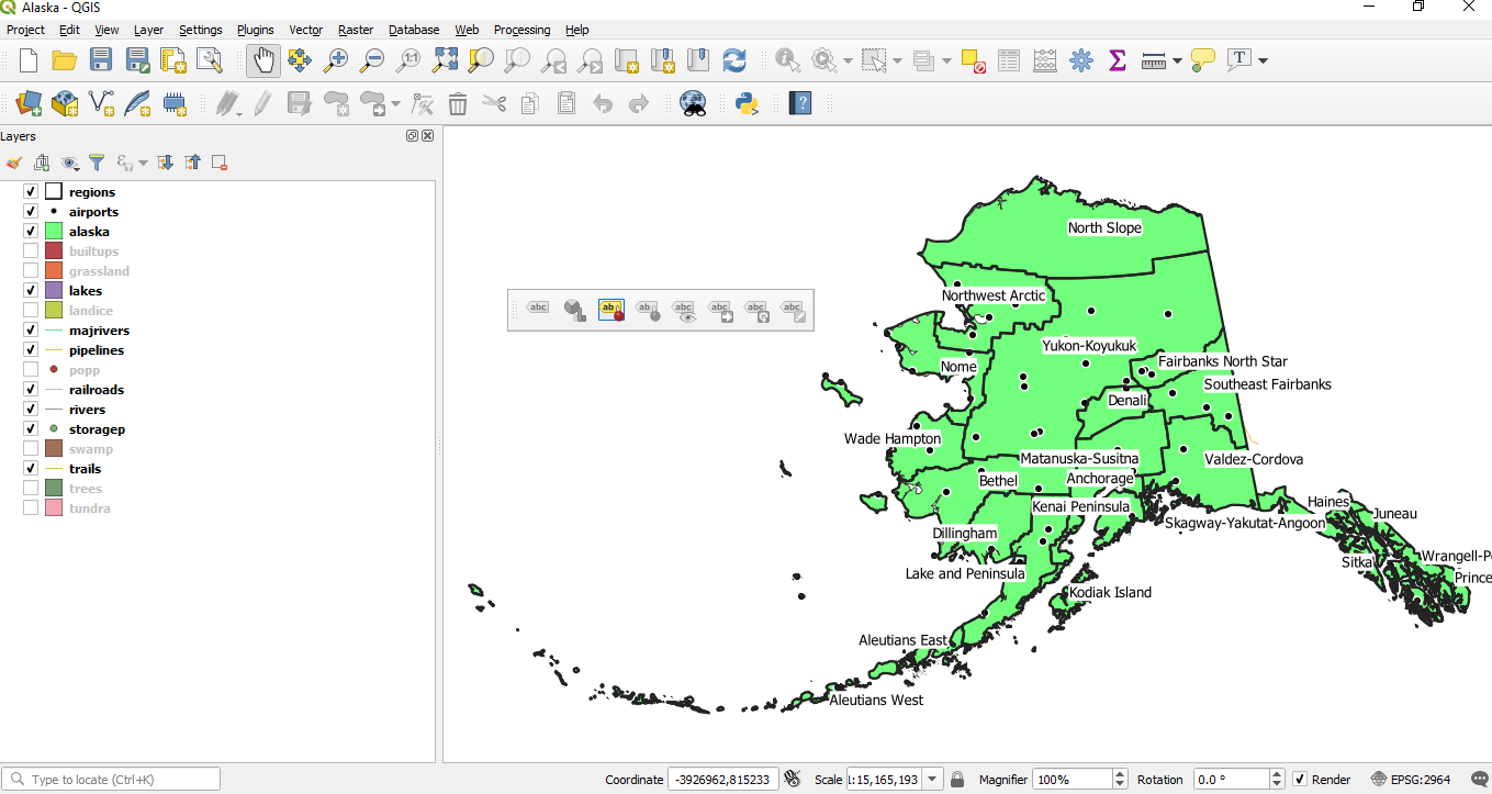
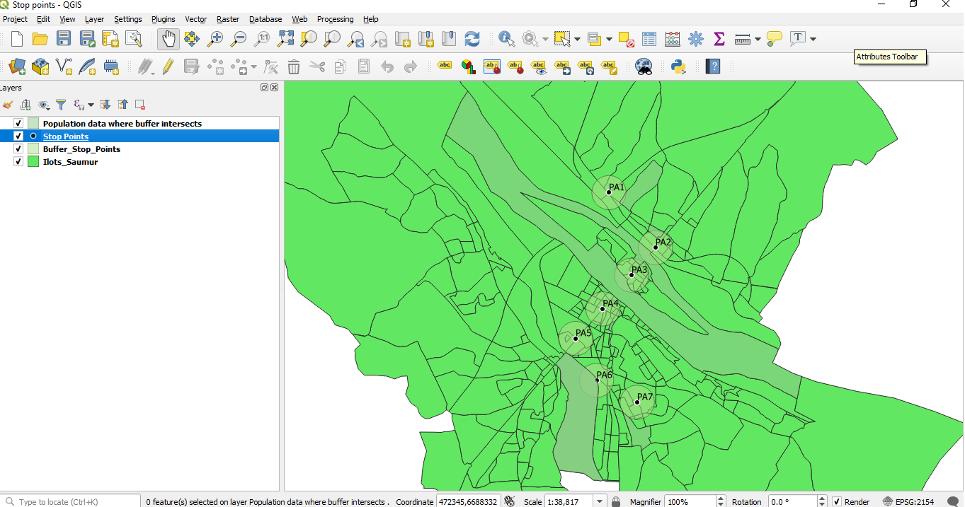
Here, I have opened a project in QGIS 3 containing layers from the Alaska data set which is available for download with the latest versions of QGIS. As you can see I have moved the Label Toolbar to the map section on this occasion for clarity purposes. Normally it would be positioned on the top menu.

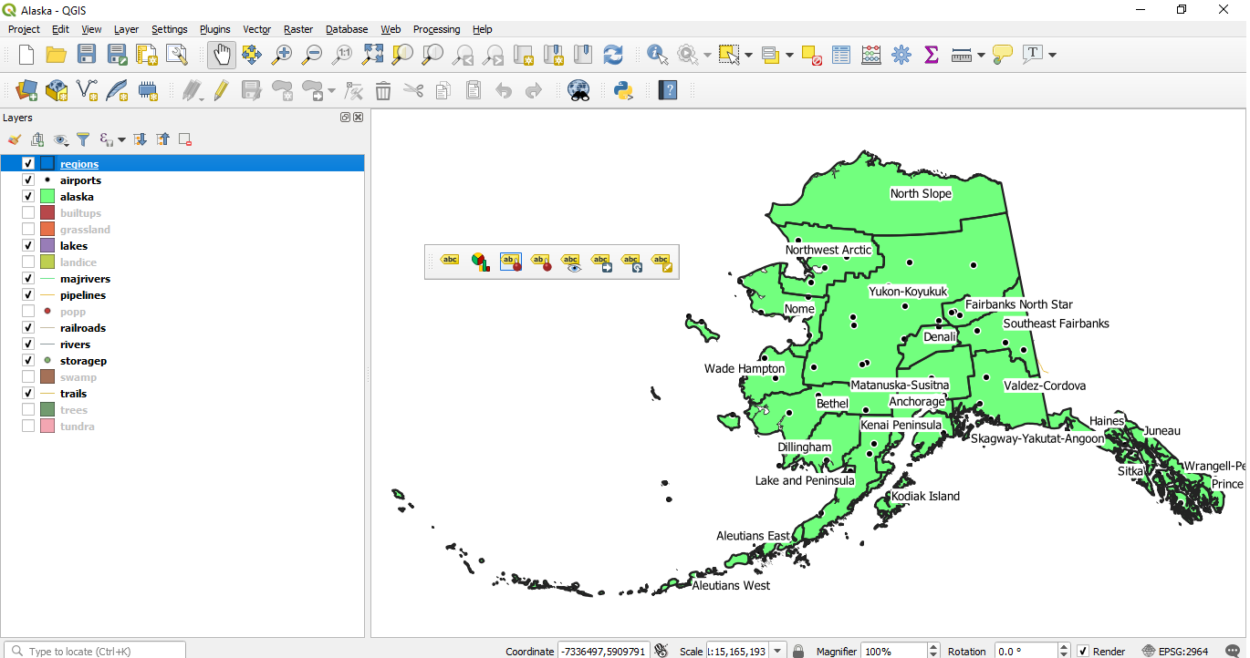
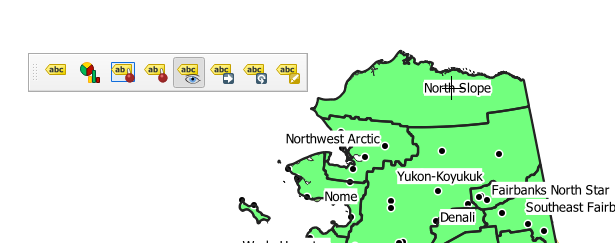
In this screen shot of the Label Toolbar only one of the icons is currently enabled. In earlier versions of QGIS, as previously discussed, most of these icons would stay greyed out without a lot of extra work being involved. However, if we now click on the regions layer in the Layers panel all of the icons will be enabled as shown in the next screen shot.

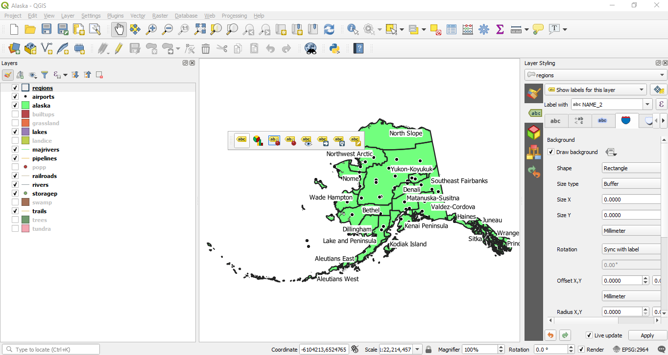
Clicking on the abc icon brings up the Layer Styling dialogue panel. As we have selected a layer with labelling enabled we have a number of options available.   

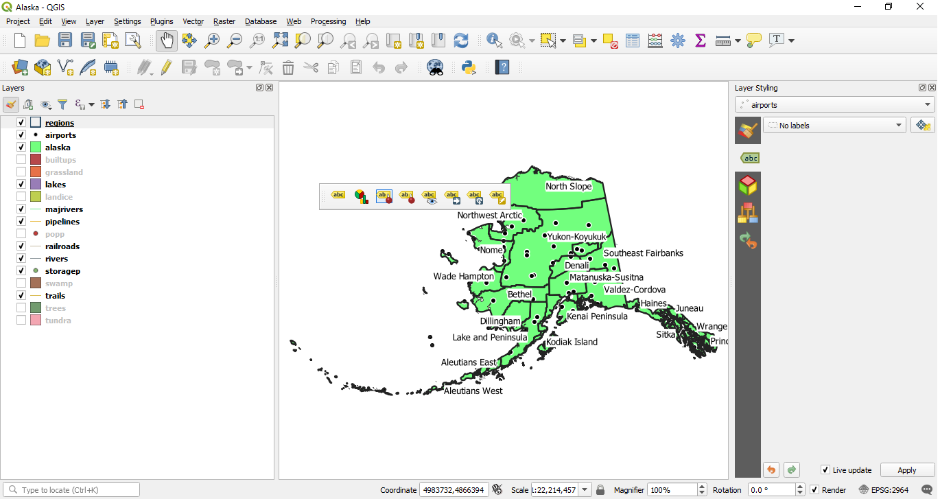
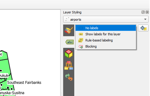
If we switch to another layer such as airports we no longer have any features enabled as shown in the next screen shot. You can do this either by selecting airports from the drop down section of Layer Styling dialogue panel or by switching from the regions to the airports layer in the Layers panel.

To create labels on a layer first you need to select the Show labels for this layer option from the drop down list as shown in the next screen shot. Then select an attribute from the layer’s attribute table to label the map with.

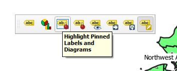
 On the Label Toolbar there are six buttons for modifying labels. Starting from the left is the Highlight Pinned Labels function which will show those labels which have been modified in some way. The cursor appears as a cross on the map when the Label Toolbar is activated.

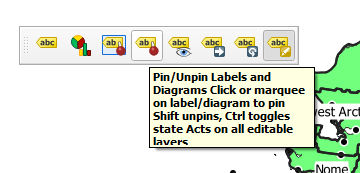
Similarly the Pin/Unpin Labels function will enable labels to be modified as well as reverted to their previous state.

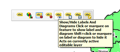
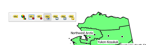
If you want to hide a label first click on the Show/Hide Labels function as shown in the next screen shot.  

 Placing the cursor over a label as in the next screen shot. The cursor is represented by a cross.

 Pressing the Shift key together with a mouse click will hide the label as shown in the next screen shot.

To hide several layers follow the above process but create a rectangle around the labels you wish to hide. Similarly, to show labels either click or create a rectangle around the area where the labels are hidden.

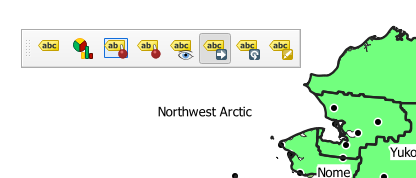
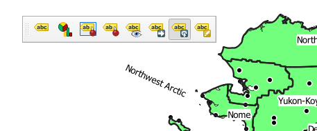
The Move Label and Diagram icon enables labels to be moved as necessary. In the next screen shot I have clicked on the Northwest Arctic label and moved it to the left.  

 Once in the desired position letting go of the mouse button will place the label in the new position.

Enabling the Rotate Label and clicking and holding down the mouse whilst rotating as desired will reposition the label.

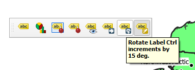
​ Here we have clicked on label and rotated it 24 degrees.

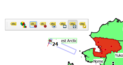
 Once the mouse is released the label will stay in its new position as shown in the next screen shot.

The Change label option allows you to modify the look of individual labels. Click on a label and the Label Properties dialogue box for the label will appear as shown in the next screen shot.

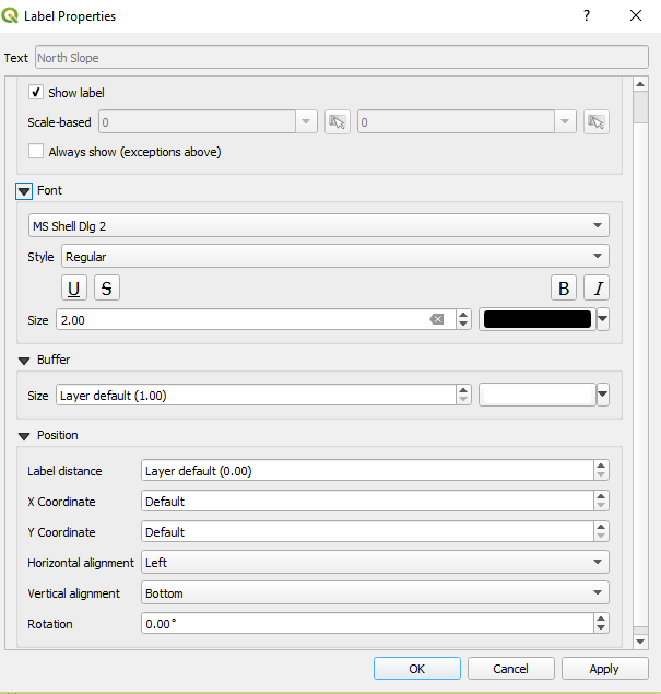
 As you can see there are numerous options for personalising specific labels with this dialogue box. This option enables a label to have a variety of changes simultaneously rather than using the individual options to move, rotate or hide.

As mentioned earlier the improvements to the labelling functions in QGIS 3 makes modifying labels a much easier task than with earlier versions of QGIS.

Geographic joins

Intersects: this geographic function compares data within two tables.

A point, line or polygon intersects another point, line or polygon when they have at least a node in common: a network crosses another network for example a road or a railway line.

The intersection means a geographical geometry touches or goes through another.

Contains and its reciprocal Within means geographical geometries are within another geometry.

A geometry A contains a geometry B when it contains the centroid of B.

When B is within A: for example a catchment area contains clients represented by point geometries.

Entirely within and its reciprocal Contains entire.

A geometry A is entirely within a geometry B when the group of nodes of A are within B.

According to the type of the compared geometry, according to needs, depends on which of these operators are chosen.

Generally, use the Intersects function to compare polygons or from polygons to lines. ​
​

The dialogue box in the Info section states that Project layers: Not connected.

In the Providers section double click on the Project layers option.

The various layers are now displayed

Click on the Ilots_Saumur option and view the Info, Table and Preview tabs​

​In the Tables drop down list choose the Ilots_Saumur and Buffer_Stop_Points tables

Click in the Columns section and from the Columns drop down list choose

Ilots_Saumur.PSDC99

Buffer_Stop_Points.ID_PA

Ilots_Saumur.geometry​

Buffer_Stop_Points.geometry

Choose Ilots_Saumur.geometry from the Columns section ​

Put a comma after this entry

Then choose Buffer_Stop_Points.geometry and add a closing bracket​

Click in the Group by section and choose Buffer_Stop_Points.ID_PA from the Columns drop down list as in the following screen shot

Click on the OK button​

Click on the Execute button or Ctrl + R

Select Load as new layer by ticking in the box

The Co-ordinate Reference System dialogue box appears. Click OK to accept the default co-ordinate system​

Name the layer as “Population data where buffer intersects” in the Layer Name section​

The layer is loaded into QGIS

If you wanted the find the population data for the areas which intersect the seven buffers we could modify the SQL as follows

This will create a new layer similar to the previous one but with a different attribute table as shown below.

With virtual layers you can create more complex SQL statements than is possible with the QGIS field calculator.  Now it is possible to use ESRI shape and MapInfo mif files to create SQL statements previously only feasible with  PostGIS, MySQL and Oracle Spatial formats.